Reproducibility in science (without getting into semantics) is the ability of other scientists to reproduce your results. The first step of that is being able to check what you have done. Did you make a mistake with your algebra? Does running the same experiment give wildly different results? As the use of computational methods in ecology increases, we are in a position where we should be able to quickly and easily reproduce the research in an entire paper. First I rerun your code, and check that the outputs match those in your paper (should be easy). Then I check the code for errors (less easy).
However, even the first step is often hampered. Code is not included in a paper, or is hidden in an unsuitable format in the supplementary material, which is hosted neither carefully nor with longevity in mind. When code is included, the data needed to run an analysis is often not. Other times, a script is included, but is a mess with different bits of analysis and output all jumbled together.
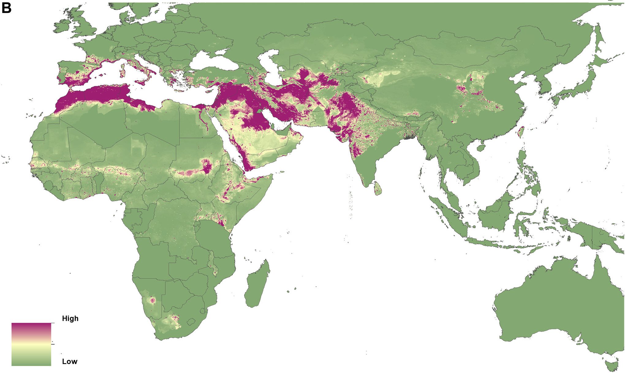
Species distribution modelling (SDM) uses data on where a species lives to predict the whole distribution of the species. In short, a species is likely to exist in areas with environmental conditions similar to those we have seen it in before. So, as long as your data is shared, I should be able to reproduce your results with minimal effort. However, even field defining papers are completely unreplicable. For example Elith et al. (2006) benchmarks how good a number of different models are and has been cited some 3,000 times. However the paper is totally unreplicable. It would be great would be to add more recently developed methods to this benchmark. If a new method can’t outperform the current ones, then it is not very useful. But with the previous benchmark being unreplicable, this is not possible.
An example use of SDM, mapping the climatic niche of leishmaniases. Pigott et al. 2014. DOI: http://dx.doi.org/10.7554/eLife.02851.007
The Internship
Over the past months I have been working on an internship creating an R package for reproducible SDMs. The package is called ZOÖN and can be found on github with more information here. The ideas behind ZOÖN have been developed over the last year, with consultation of SDM users at every step (i.e. before I started). It is hoped that this constant discussion will avoid pitfalls of writing software that is then never used. It was decided that while there are great SDM packages out there (biomod2, maxent etc.) there was still a gap for a higher level package, that aids the running, sharing and reproducing of whole SDM analyses, including data collection, data cleaning and outputs. However, as this is a fast moving field, an inflexible package, written and maintained by a small group of developers, would quickly become out of date. So instead the plan is to use web-hosted ‘modules’ that are quick and easy to program (compared to a full R package). ZOÖN will pull these modules from the web and run an analysis. This also means wrappers for other packages can easily be written.
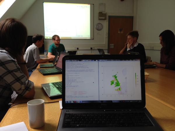
Presenting the package at a workshop
The goal of the internship was to write a working prototype R package which I think I have succeeded in. The working package is on github and can be installed in R with devtools::install_github("zoonproject/zoon"). Although there is some work to be done, the core package works. Whole SDM workflows can be run with one command. The output then contains all the data needed to run the analysis and a record of the call (the inputted text command) used to run the analysis. As the modules are all online, an analysis can be rerun simply be having access to this output (one R object.) In the case of analyses using online data (from GBIF for example) only the call is needed to rerun an analysis. Furthermore, while still in early development, there is already a very simple way to upload an analysis to Figshare.
To run a SDM with the package you must specify at least five ‘modules’. One each that: collects occurrence data, collects environmental data, processes the data, runs a model, gives some output. To flesh out the variety of analyses possible will require much more work writing modules (there are plans for a hackathon to get this going.) However, as wrapping existing packages is easy, there are already modules for running all the models available in Biomod2, collecting data from GBIF, worldclim and NCEP and creating basic maps and uploading analyses to Figshare to name a few.
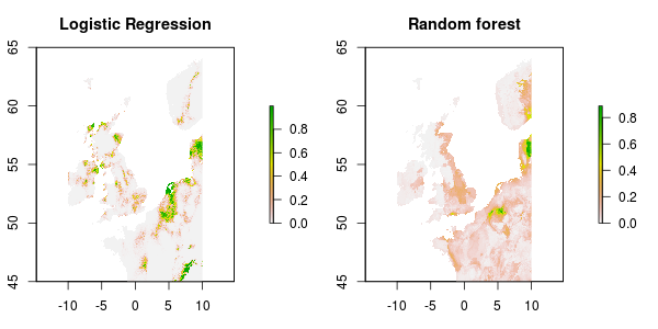
Two distributions of Eresus sandaliatus created using ZOÖN
So in three months I think I have laid the ground work for a package that really simplifies sharing analyses while making it easy for new methods to be incorporated into current analyses.
Open science
This project has been conducted in a very open manner which I have really enjoyed. The code can be found on github as soon as it is written. And the code is licensed to make it useable by anyone. Most of us areontwitter and happy to discuss the research. And as discussed above, regular contact with a user panel means we are not locked in our dark computer lab, working in isolation.
Lessons
Through this internship I have learned an awful lot about the nuts and bolts of R. Writing a package is a really good way to get to know the language better. I can totally recommend R packages and Advanced R for more information.
I have also become much more comfortable with handling a large (ish) software project. Git is now second nature, using Github to record issues has become an invaluable tool and the benefits of unit testing have become clearer.
On a less tangible front it has been really interesting to see how differently people approach approach the community side of software development. Without users, your software is worthless. This project relies on it’s community for more than just a user base. We are hoping for users to contribute code in the form of modules. So community development has been important from the beginning. However I really liked working while talking to potential end users (although a workshop six weeks into a project is terrifying.) I don’t think this approach is easy, but I definitely think it’s worth putting effort into building a community around your software.
And now it just remains to see how the project develops and whether the software becomes commonly used.
A practical guide to squishing yearly ‘disag data’ objects
A practical guide to pooling annual data for Bayesian disaggregation regression in R
This post is a guest post by my predoctoral fellow, Samana.
Bayesian spatial disaggregation gives you a high resolution risk surface from low-resolution case counts ….. but only one year at a time. This post shows how to pool several years into a single model fit.
Hi all, my name is Samana and I’m a predoctoral fellow and I’ve been working on the problem of a multi-year disaggregation model!
In this blog I will be presenting a recipe of how to do a multi-year disaggregation model fit.
Currently, using the disaggregation package we can only really fit one model per time slice of data we might have, but this blog aims to change that and let you fit a disag model with multiple years of data.
Part A demonstrates the mechanics without a time trend; Part B adds a time spline to the six-year model. This blog is part A.
This post shows how to combine annual disag_data objects and fit one pooled spatial disaggregation model. It demonstrates shared effects across years and it is not a full spatio-temporal model with separate spatial field for each year.
The resolution mismatch problem:
Simply put, there is a resolution mismatch between satellite covariates (which are very high resolution) and public health data, like case counts of a particular disease in a specific county (this is low resolution).
Public health data is often reported as annual case counts for administrative areas such as counties and districts whereas environmental information that may explain risk, such as temperature, land cover, vegetation is often available on a fine spatial grid.
The problem is that we can’t just combine these together and then fit a model for risk predictions to get a high resolution risk surface. This is because of the ecological fallacy.
These figures above show the resolution mismatch; on the left we have the low resolution public health case counts and on the right we have the high resolution environmental satellite covariates (Nandi et al. 2023, https://doi.org/10.18637/jss.v106.i11).
What is disaggregation and why you’d want to do it:
So these resolutions are linked by modelling a latent disease risk at the pixel level and THEN aggregating the pixel level predictions to the polygon level so they’re consistent with the observed disease counts. all of this is done by Bayesian spatial disaggregation (implemented in the R package disaggregation )
The package fits a Bayesian disaggregation regression model (similar to a GLM) with an INLA style spatial random field via TMB, using the function prepare_data() to line up polygons, covariates and population, and disag_model() to fit the model.
The current single year workflow is like this:
Read in the inputs: a sf object containing the area boundaries and case counts, a SpatRaster of fine-scale covariates, and a population raster when modelling counts with population as exposure.
Prepare these inputs into a coherent data object with prepare_data().
Fit the model with disag_model(), choosing the likelihood and link and whether to include a spatial field and an independent (iid) effect.
Inspect the fit with summary() and plot(), then use predict() to produce fine-scale prediction and uncertainty maps.
For multiple years, the missing step is between 2 and 3: prepare each year separately, then combine the resulting disag_data objects carefully before fitting one pooled model.
Why multi-year disaggregation?
When you have many years of polygon level counts, a natural question is: fit each year separately, or pool several years into one model?
Pooling helps when you want the spatial field and covariate effects to borrow strength across years, while still letting a time trend move through a flexible term (we’ve used a natural spline on centered year in part B of this blog).
I’ve been calling this “squishing” years together, stacking each year’s prepared data into one long object before handing it to disag_model().
Bayesian spatial disaggregation is straight forward for one year of data but multi-year models are harder because the disag_data object contains many components that need to be in the right shape, format and size.
This object contains polygon-level outcomes, pixel-level covariates, aggregation weights, spatial coordinates, start end indices and the spatial mesh. These objects must remain correctly aligned when the years are combined.
This tutorial develops a reproducible workflow for combining yearly disag_data objects informally, “squishing” or “combining” them before fitting a multi-year Bayesian disaggregation model.
Model components
The disaggregation regression models demonstrated here include fixed effects of covariates and a number of random effects, for various different modelling purposes.
In this example, the pooled model estimates shared climate effects. We have different covariate observations for each year, but want to fit a model using all years of data in one go.
The spatial random effect operates at high resolution. If you model each year separately, then each time period has its own spatial field, defined over the mesh and projected to the pixels. It captures smooth residual spatial variation that remains after accounting for measured environmental covariates. However, we often want to pool estimates for this random effect across years.
The iid random effect operates at polygon level, the lower resolution. It gives each polygon-time observation an additional independent residual term, helping account for overdispersion and unmeasured area-level factors.
When yearly data are squished, the model is fitted jointly across all periods. The workflow must preserve the relationships between each polygon, its pixels, its aggregation weights and its appropriate spatial field.
The iid term allows an additional residual effect for each polygon-year observation. Stacking the data does not automatically create a separate spatial field for each year or model how fields evolve over time.
THE DATA:
The example region is Madagascar, deliberately chosen because it’s the same country used in the disaggregation package’s own founding methods paper (Nandi et al. 2020, malaria case counts across Madagascar, [Nandi et al](https://www.jstatsoft.org/article/view/v106i11)) so the mesh settings and covariate naming are the same as that original worked example.
The geometry, climate covariates AND population is real public data; only the case counts are simulated (real disease data can’t be shared here for data-permission reasons)
The dataset pairs real, public district geometry, real climate covariates and real population with simulated case counts:
Real public administrative level-2 (district) boundaries for Madagascar, from the GADM database (https://gadm.org), downloaded via the R geodata package.names.
Year varying covariates (temp_wc, precip_wc): annual mean temperature and annual total precipitation for each simulated year, built from REAL monthly TerraClimate records (Abatzoglou et al. 2018) not long-run climate normals, so these differ from one year to the next. Centred and scaled (mean 0, sd 1, using one mean/sd computed across all years combined so real year-to-year differences are preserved). Source: https://www.climatologylab.org/terraclimate.html.
Simulated case counts drawn from known truth parameters (shipped alongside the data as true_parameters.csv), using the real covariates and population above plus a simulated spatial random field and district-level noise. So this post can check whether the fitted model recovers the true coefficients, a much better teaching device than fitting to arbitrary noise.
None of the numbers in the dataset correspond to any real disease case count.
:::
### Step 4: prepare data for each year
Mesh args here match those used in the `disaggregation` package's own
Madagascar malaria worked example (Nandi et al. 2020) a nice side
benefit of picking the same country is that these don't need retuning
from scratch.
Always retune these to your own study area if you swap in a different
region.
The details for what these parameters mean can be found in the inla
tutorials for example.
::::::: cell
``` {.r .cell-code}
mesh_args_mdg <- list(max.edge = c(0.7, 8), cutoff = 0.05, offset = c(1, 2))
dis_2001 <- prepare_data(
polygon_shapefile = shapes_2001,
covariate_rasters = cov_stack_2001,
aggregation_raster = population_raster,
mesh_args = mesh_args_mdg,
id_var = "district_id",
response_var = "cases",
na_action = TRUE
)
::: {.cell-output .cell-output-stderr} Warning: [rast] CRS do not match :::
::: {.cell-output .cell-output-stderr} Warning: [extract] transforming vector data to the CRS of the raster :::
::: {.cell-output .cell-output-stderr}
Warning: [rast] CRS do not match
Warning: [extract] transforming vector data to the CRS of the raster
:::
``` {.r .cell-code}
dis_2003 <- prepare_data(
polygon_shapefile = shapes_2003,
covariate_rasters = cov_stack_2003,
aggregation_raster = population_raster,
mesh_args = mesh_args_mdg,
id_var = "district_id",
response_var = "cases",
na_action = TRUE
)
::: {.cell-output .cell-output-stderr} Warning: [rast] CRS do not match Warning: [extract] transforming vector data to the CRS of the raster ::: :::::::
Step 5: The squish: stack the 3 years of data into one disag data object
To stack these objects together correctly, we handle different parts of the data differently. polygon_data and covariate_data are just stacked with a year label attached. We offset start_end_index: each prepare_data() call starts its pixel-row numbering again, so the second and third years’ indices must be shifted to point to their new positions in the combined covariate table.
::: cell ``` {.r .cell-code}
polygon_data and covariate_data just stack with a year label attached
poly_0103 <- bind_rows( transform(dis_2001$polygon_data, year = 2001), transform(dis_2002$polygon_data, year = 2002), transform(dis_2003$polygon_data, year = 2003) )
cov_0103 <- bind_rows( transform(dis_2001$covariate_data, year = 2001), transform(dis_2002$covariate_data, year = 2002), transform(dis_2003$covariate_data, year = 2003) )
:::
### step 6: fit the pooled model
:::::: cell
``` {.r .cell-code}
fit_0103 <- disaggregation::disag_model(
data = dis_0103,
iterations = 1000,
field = TRUE,
iid = TRUE,
family = "poisson",
link = "log"
)
::: {.cell-output .cell-output-stderr} Fitting model. This may be slow. :::
Compare that against three separate single-year fits (disag_model() on 2001, 2002, 2003 individually, no squishing) to see whether pooling changes the covariate estimates, tightens their standard errors, or shifts the spatial field. This comparison is the actual point of the exercise the code above just gets you to a model you can compare against.
:::::: cell ``` {.r .cell-code} fit_2001 <- disaggregation::disag_model(dis_2001, iterations = 1000, field = TRUE, iid = TRUE, family = “poisson”, link = “log”)
::: {.cell-output .cell-output-stderr}
Fitting model. This may be slow.
:::
``` {.r .cell-code}
fit_2002 <- disaggregation::disag_model(dis_2002, iterations = 1000, field = TRUE,
iid = TRUE, family = "poisson", link = "log")
::: {.cell-output .cell-output-stderr} Fitting model. This may be slow. :::
``` {.r .cell-code} fit_2003 <- disaggregation::disag_model(dis_2003, iterations = 1000, field = TRUE, iid = TRUE, family = “poisson”, link = “log”)
::: {.cell-output .cell-output-stderr}
Fitting model. This may be slow.
:::
::::::
::::::: cell
``` {.r .cell-code}
summary(fit_2001)
Pooling the three years reduced uncertainty: the pooled model had smaller standard errors for both temperature and precipitation than any separate annual model. The temperature estimate was positive and the precipitation estimate negative, consistent with the values used to simulate the data.
Refrences
Nandi, A., Lucas, T., Arambepola, R., Python, A. (2023). disaggregation: An R Package for Bayesian Spatial Disaggregation Modeling. Journal of Statistical Software, 106(11). https://doi.org/10.18637/jss.v106.i11
Nandi, A., Lucas, T., Arambepola, R., Gething, P., Weiss, D. (2020). disaggregation: An R Package for Bayesian Spatial Disaggregation Modelling (original methods paper, Madagascar malaria worked example). https://arxiv.org/abs/2001.04847
GADM database of global administrative boundaries: https://gadm.org
Abatzoglou, J.T., Dobrowski, S.Z., Parks, S.A., Hegewisch, K.C. (2018). TerraClimate, a high-resolution global dataset of monthly climate and climatic water balance from 1958-2015. Scientific Data, 5, 170191. https://doi.org/10.1038/sdata.2017.191